Demystifying MediaPipe's selfie segmentation model

Stand on the shoulders of giants, right?

As you may know, I’ve just started a side quest to develop a Bayesian portrait segmentation algorithm. One of my early tasks was to:

… familiarise myself with the design of MediaPipe’s selfie segmentation model.

I plonked it into netron.app to have a peek under the hood and this was what I saw:

That’s quite the network!

Clearly there are some building blocks, but the number and type of block has likely been determined by some learning process - there’s just too many for this to be hand made! According to the model card, the architecture is:

MobileNetV3-like with customised decoder blocks for real-time performance.

Off I went and read through the publication behind MobileNetV3 by Howard et al, 2019 (there’s also a pre-print), and this confirmed my suspicion: the network was learned.

What was really kicking my arse, though, was the volume of technical jargon used to explain the research. So let’s demystify and experiment with a few fundamentals!

1. What ’neural networks’ are used in image segmentation?
2. What does a ‘convolution’ look like?
3. What do ‘features’ look like in context of MobileNetV3/MediaPipe’s portrait segmentation?
4. How does MediaPipe/MobileNetV3 generate a probability for person vs background?

Neural networks in image segmentation

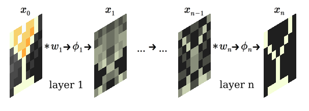
First, and possibly foremost, the dominant algorithms are ‘feed forward convolutional neural networks (CNNs)’. At their simplest, these take an input image, denoted \(x_0\), and calculate a sequence \(x_1, \ldots x_n\) using a convolution-like operator, denoted \(\star\), with weights \(w_1, \ldots, w_n\), and activation functions \(\phi_1, \ldots, \phi_n\):

Each step in the sequence is typically called a ’layer’, that is, the operation going from \(x_{i-1}\) to \(x_i\) describes one layer. A schematic of a CNN that segments an image of a cocktail glass 🍸️ might look like:

Convolution of an image

By way of introduction, a convolution operator might look a lil’ something like this (to a mathematician):

Speaking more conceptually, and in context of image segmenation, consider the convolution in the first layer:

• For each channel (usually red [R], green [G], and blue [B]) of the image (the input):
  • Move the kernel ‘window’ over the \((i, j)^\text{th}\) pixel.
  • For each pixel, indexed by \((m,n)\), in the window: take the product of the kernel and the value in the channel i.e. calculate \(x_0[i-m, j-n] w[m, n]\) for each \(m\) and \(n\).
• Take the sum over all channels of all the products obtained to determine the \((i,j)^\text{th}\) pixel in the output, i.e. do \(\sum_{m,n}\).

Let’s visualise this using a convolution of an 8x8 (RGB) image of a cocktail glass 🍸️ with an 8x8 result:

• The input, the 8x8 cocktail glass image, is shown on the left.
• The R, G, and B channels are shown explicitly in the next column.
• A randomly generated 2x2x3 kernel is displayed, each channel separately, in the next column.
• The final (8x8x1) convolution is shown, in grayscale, on the right.
• The window of the kernel moves over the image (or each channel), demonstrating the source of the data for each pixel in the result.

Now, I said earlier that image segmentation algorithms use convolution-like operators because:

• OpenCV is very explicit that their filter2D function does not perform a typical convolution by default.
• Keras is not specific with regards to Conv2D; it turns out its essentially the same as OpenCV (code snippets are included in Appendix: Bonus comparisons).
• Some layers will also perform downsampling. That is, instead of computing the convolution-like value for every pair \((i, j)\), it is computed for every 2^nd pair of \(i,j\) to reduce the width and height by a factor of two (or every 4^th etc).

Because of the fuzziness about the term ‘convolution’, a comparison of the mathematical definitions is provided in the Appendix: Convolution operators (consult at your own risk).

Featuring: features

The output from each layer (particularly the first layer) is often a set of ‘features’. In most image segmentation architectures, certainly with MobileNetV3, the first layer extracts a number of features by using different kernels on the image. Let’s taker a closer look at MediaPipe’s first layer in netron:

• input_1 is the (RGB) image, given as a 1x144x256x3 ’tensor’.
• Conv2D is Keras’ 2D convolution layer with two key inputs: bias and kernel (weights).
• Two Dequantize nodes represent the bias and kernel (weights) inputs.
• The kernel input has shape 16x3x3x3, i.e.:
  1. There will be 16 features, and;
  2. Each feature is based on a 3x3x3 kernel, i.e. the RGB channels get squashed down to one channel in each feature.
• HardSwish is the non-linear activation function given by \(\phi(x) = x \operatorname{ReLU6}(x + 3) / 6\) (see Howard et al, 2019 or Keras’ hard SiLU).
• Not shown: the convolution layer has stride attribute (equal to 2) which results in downsampling ⇒ the output tensor is 1x72x128x16.

netron allows us to export the bias and kernel weight inputs as numpy arrays. So let’s take my portrait (captured via Logitech C270) …

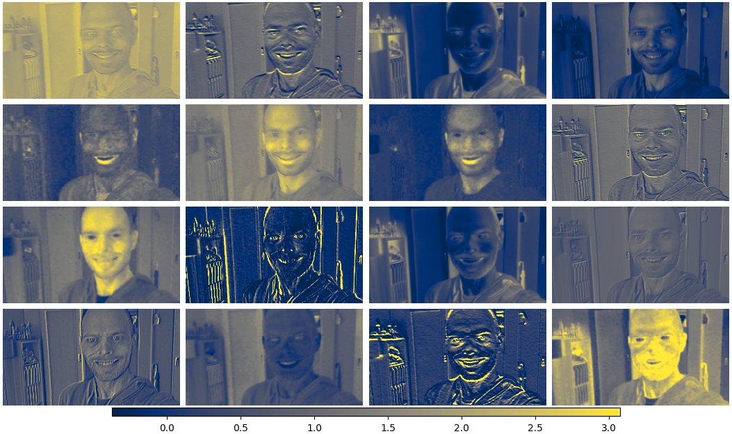
… and then summon nightmare-fuel and demons - i.e. generate the 16 features using either OpenCV or Keras (plotted using seaborn):

It’s somewhat fascinating what it has come up with. Some of the features look ’edge detection’-like, some focus mostly on one colour, a few pick out my bottom lip, and one (top right) seems to do not much at all. To my eye, some even appear redundant.

Asisde: code to generate these features is supplied here.

Aggregation and segment prediction

We’re going to skip the middle part of MobileNetV3/MediaPipe’s network, and instead look at what happens when the features are brought together in the last layer to construct a probability of ‘person’ vs ‘background’. Here’s that layer thanks, again, to netron:

• The 1x72x128x16 input coming from the top left represnts 16 transformed features that are the output of the \({n-1}^\text{th}\) layer.
• Convolution2DTransposeBias is a MediaPipe specific layer, it is an optimised implementation of Keras’ Conv2DTranspose; it also has bias and kernel inputs.
• The kernel is a 1x2x2x16, meaning that it combines 16 features into 1 final feature (or channel).
• The output is passed through the logistic function to get a probability in the interval \((0, 1)\).
• Not shown: The layer has a stride attribute (equal to 2), which performs upsampling ⇒ the output tensor is 1x144x256x1.

This layer is called a ’transposed convolution(al)’ layer (originally these were mistakenly called ‘deconvolution(al)’ layers 😖). Some prefer the name ‘convolution transpose’.

I’ve provided some mathematical details for the transposed convolution in Appendix: Convolution operators 📝. In brief, if the convolution operator is represented as a matrix \(W\) (see § Representation as a matrix multiplication) then the convolution is a particular sub-matrix of \(W^T\).

Let’s visualise one of these layers, with a stride length of 2, to demonstrate the convolution tranpose with upsampling for 4x4 features, with 3 features being combined into 1 output channel:

• The three 4x4 input features are shown on the left (colorised).
• For visual purposes only: a zero-interleaved buffer is shown in the next column to demonstrate the ‘stride’.
• A randomly generated 2x2x3 kernel is displayed, each channel separately, in the third column.
• The final (8x8x1) transposed convolution is shown, in grayscale, on the right.

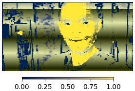
Returning to MediaPipe, I was wondering 🤔. What would happen if I skipped almost all the intermediate layers, and passed the features into the final layers 👀

Obviously, this is performing terribly, because the weights were not trained for when the model was gutted like this.

But this is a nice spot to pause.

Final remarks

There is some way to go, but much of the conceptual building blocks are falling into place. In particular we have covered the typical schema of a feed-forward neural network used in image segmentation that includes:

1. Convolutional and ’transposed convolutional’ layers.
2. ‘Feature extraction’ and downsampling that typically occurs in the first layer.
3. The aggregation of features and upsampling that occurs in the final layer.

What we haven’t covered, and what I’m interested in looking at next is:

1. The other layers in the network, which include ‘separable’ convolution operators that are described in Howard et al, 2019 - what do they achieve?
2. What exactly is optimised when the network is trained as outlined in Howard et al, 2019?
3. Can I train on my laptop?
4. Which parts of the algorithm take the most time and is there any evidence of redundant features?
5. What are some other key drivers of performance? As already discovered, MediaPipe uses a custom operator for performance, what impact does this have? What is ‘quantisation’?

‘Til next time 👋

References

Howard, A., Sandler, M., Chen, B., Wang, W., Chen, L. C., Tan, M., … & Le, Q. (2019). Searching for MobileNetV3. In 2019 IEEE/CVF International Conference on Computer Vision (ICCV) (pp. 1314-1324). IEEE. doi:10.1109/ICCV.2019.00140.

Appendix: Code to generate features

import cv2
import keras
import numpy as np

# read image and resize to 256x144
img_capture = cv2.imread('logitech_c270_capture.png')
img_capture = cv2.resize(img_capture, (256, 144))

# read the numpy array files generated by netron's export feature for inputs
mp_selfie_kernel = np.load('conv2d_Kernel')
mp_selfie_bias = np.load('conv2d_Bias')
# fix the dimension of the weights
mp_selfie_kernel = np.transpose(mp_selfie_kernel, (1, 2, 3, 0))

# define a single-layer model with hard-swish activation and set the weights
model = keras.models.Sequential()
model.add(keras.Input(shape=img_capture.shape))
model.add(
    keras.layers.Conv2D(16, (3, 3), activation='hard_silu', padding='same',
                        use_bias=True)
)
model.set_weights([ mp_selfie_kernel, mp_selfie_bias ])

# predict the features of the input image
features = model.predict(
  # NOTE: add a dimension at the start of input to get 1x144x256x3 tensor
    np.expand_dims(img_capture, axis=0).astype(np.float32) / 255
)

Appendix: Convolution operators

In the following we will start with an input \(x\) which is defined as:

where the image has width \(i_w\) and height \(i_h\). In other words, \(x\) is a zero-padded image. Note: the \(i\) index refers to the row (‘y’ axis in cartesian coordinates), and \(j\) refers to column (‘x’ axis).

The kernel could be an arbitrary function, but we’ll constrain it so that it also has a width, \(k_w\), and a height, \(k_h\), and an anchor given by the pair \((m_\text{a}, n_\text{a})\), such that:

With this in place, the result of the ordinary convolution with an output the same size as the original unpadded image is:

for \(i \in \{ 0, \ldots, i_h - 1 \} \) and \(j \in \{ 0, \ldots, i_w - 1 \}\).

For convolutional neural networks, however, the most commonly used operation is instead:

Up to this point, the equations are for the unit-stride case (stride equal to one). To perform downsampling, we introduce stride height, \(s_h \ge 1\), and stride width, \(s_w \ge 1\), and define the output as:

for \(i \in \{ 0, \ldots, \lfloor i_h / s_h \rfloor - 1 \} \) and \(j \in \{ 0, \ldots, \lfloor i_w / s_w \rfloor \} - 1\). This is conceptually the same as computing every \({s_w}^\text{th}\) value of the convolution on the horizontal axis, and every \({s_h}^\text{th}\) on the vertical axis, with some adjustment for the index in the output.

Representation as a matrix multiplication

As a bridging step between the operation of a ‘convolutional layer’ and the operation of a ’transposed convolutional layer’: consider the 1-dimension case with unit stride:

Let \(x\) be the padded column vector and \(y\) be a column vector of output, i.e.:

and define the matrix \(W\) such that \(W_{i,m} = w[m-i] \), i.e.:

Then the convolution is a plain old matrix multiplication:

To incorporate stride (downsampling), keep only the first \(\lfloor n / s_h \rfloor \) rows, and shift the values in the \(i^\text{th}\) row to the right by \(s_h \times i\) (inserting zeros on the left), e.g. for an input of length 6, a kernel of size 2 anchored at 0, downscaling by a factor (stride) of 2:

Transposed convolutional layer

Piggy-backing off the definition of the operation as a matrix, consider taking the transpose of \(W\) with unit stride:

Typically, this isn’t quite what we want, rather we want an output that is the same size as the (unpadded) input; so the first \(m_a\) rows and the last \(k_h - m_a - 1\) rows are dropped from the transpose. And thus, the ’transposed convolutional layer’ is born.

Upsampling is obtained by considering the \(W\) operator for an input with the upscaled size using the upscale factor as the stride, and then taking the transpose; that is, to upscale an input of size 3 by a factor (stride) of 2, with a kernel of size 2 anchored at 0:

We essentially work backwards to recover a formula for the operation of a transposed convolutional layer for a two-dimensional image. In the unit-stride case we have:

This is, surprisingly, an ordinary convolution.

In the non-unit stride case the output is:

for \(i \in \{ 0, \ldots, s_h \times i_h - 1 \}\) and \(j \in \{ 0, \ldots, s_w \times i_w - 1 \}\).

This wasn’t an exhaustive description of the possible configurations of these layers. For example, Keras layers have:

1. A dilation attribute that performs the opposite role to the stride attribute.
2. An alternative padding scheme (called 'valid') that results in a different (size) output to the zero-padded scheme we’ve covered here.

None the less, this should provide some of the basic footwork.

Appendix: Bonus comparisons between OpenCV and Keras

In constructing these demonstrations, I first turned to OpenCV as it has simpler and better-documented syntax for loading images and transforming them compared to Keras.

However, I ultimately needed to cross-check that I was understanding the layers in Keras correctly, sand hence these code snippets demonstrate how to reproduce Keras’ convolutional and transformed convolutional layers using OpenCV.

I only considered the padding='same' case; the non-padded case would (likely) follow with some minor adjustments.

For each demonstration, we’ll start with the following randomly generated input tensor and set the kernel width (and height):

import numpy as np
np.random.seed(451)
x = np.random.rand(1, 12, 24, 1) # input noise
k_w = 4                          # kernel size

Convolutional layers

For convolutional layers, it is relatively straightforward to reproduce using OpenCV. Simply call cv2.filter2D with:

• borderType equal to cv2.BORDER_CONSTANT, and;
• anchor equal to (k_w - stride) // 2.

Caveat: modifications needed if the input dimensions are not a multiple of the stride.

import cv2
import keras

# downscaling factor a.k.a. stride in the layer
stride = 2

# set python seed to get reproducible weights
import random
random.seed(451)

# define convolutional layer in Keras with a pass-through activation function
y = keras.layers.Conv2D(1, (k_w, k_w), strides=stride,
                        activation='linear', padding='same')
# initialize and retrieve weights for the layer
y.build(x.shape)
kernel = np.squeeze(np.asarray(y.weights[0]))
bias = np.asarray(y.weights[1])
# get ouput of layer from keras
z_keras = np.squeeze(y(x))

# filter
anchor = (max(0, (k_w - stride) // 2), ) * 2
z_cv2 = cv2.filter2D(np.squeeze(x), ddepth=-1, kernel=kernel,
                     anchor=anchor, borderType=cv2.BORDER_CONSTANT)
# downscale (requires input lengths are mutiple of stride)
z_cv2 = cv2.resize(z_cv2, dsize=None, fx=1 / stride, fy=1 / stride,
                   interpolation=cv2.INTER_NEAREST)

# mean difference
print(np.mean(z_keras - z_cv2))

Transposed convolutional layers

The tranposed convolutional layer also turns out to be relatively straightforward to replicate using OpenCV. The input first needs to be zero-interleaved for upscaling, then flipped, then passed to filter2D. The result is then flipped (again). Just like a convolutional layer, filter2D needs to be called with the following arguments:

• borderType equal to cv2.BORDER_CONSTANT, and;
• anchor equal to (k_w - stride) // 2.

# upscaling factor a.k.a. stride in the layer
stride = 2

# could reset RNG if you want here

# define transposed convolutional layer with a pass-through activation function
y = keras.layers.Conv2DTranspose(1, (k_w, k_w), strides=stride,
                                 activation='linear', padding='same')
# initialize and retrieve weights for the layer
y.build(x.shape)
kernel = np.squeeze(np.asarray(y.weights[0]))
bias = np.asarray(y.weights[1])
# get ouput of layer from keras
z_keras = np.squeeze(y(x))

# create an upscaled buffer with interleaved zeros
buffer = np.zeros(z_keras.shape[:2])
buffer[::stride,::stride] = np.squeeze(x)

# flip, filter, then flip
anchor = (max(0, (k_w - stride) // 2), ) * 2
z_cv2 = np.flip(
    cv2.filter2D(np.flip(buffer), ddepth=-1, kernel=kernel,
                 anchor=anchor, borderType=cv2.BORDER_CONSTANT)
)

# mean difference
print(np.mean(z_keras - z_cv2))

Cross-check mathematical formula

Lastly, given the output from the preceding snippet, we can test the formula provided earlier for a transposed convolutional layer:

in_x = np.squeeze(x)
z_blog= np.zeros(tuple(stride * value for value in in_shape))

# inefficient but correct loop
for (i, j) in itertools.product(range(stride * in_x.shape[0]),
                                range(stride * in_x.shape[1])):
    for (m, n) in itertools.product(range(k_w), range(k_w)):
        M = (i - m) // stride
        if (M >= 0) and ((i - m) % stride == 0): # and M < in_x.shape[0]:
            N = (j - n) // stride 
            if (N >= 0) and ((j - n) % stride  == 0): # and N < in_x.shape[1]:
                z_blog[i, j] += in_x[M, N] * kernel[m, n]

# mean difference between keras and formula at <stephematician.gitlab.io>
print(np.mean(z_keras - z_blog))